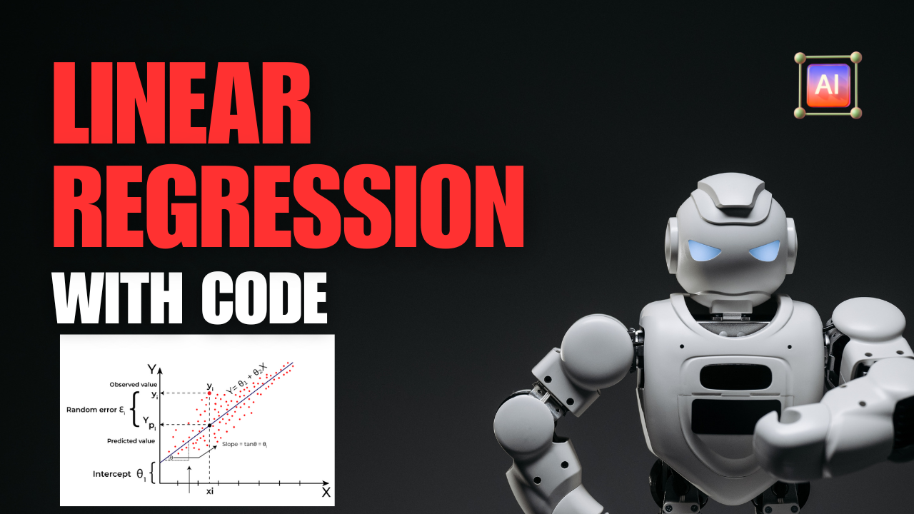
Linear regression is one of the simplest and most popular machine learning algorithms used for predicting a continuous target variable. It is based on the idea of fitting a straight line through a dataset, where the line represents the relationship between the input features (independent variables) and the target variable (dependent variable).

In this blog, we’ll explore the fundamental concepts of linear regression, work through a real-life example, and implement it using Python.

What is Linear Regression?

Linear regression is a supervised learning algorithm used for regression tasks. It models the relationship between the dependent variable (target) and one or more independent variables (features) by fitting a linear equation to the data. The equation for simple linear regression (with one independent variable) is:

How Linear Regression Works

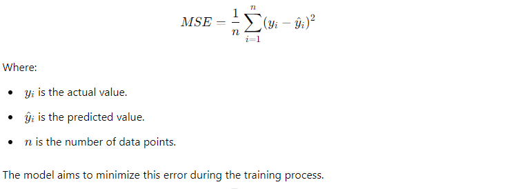
The goal of linear regression is to find the best-fitting line that minimizes the difference (error) between the predicted values and the actual values in the training data. This is achieved using the Ordinary Least Squares (OLS) method, which minimizes the sum of squared residuals (the difference between observed and predicted values).

The loss function for linear regression is typically Mean Squared Error (MSE), given by:

Real-Life Example of Linear Regression: Predicting House Prices

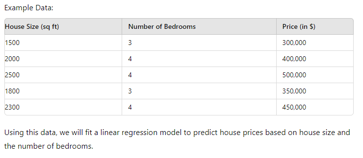
A common real-life example of linear regression is predicting house prices based on various factors like the size of the house (square footage), the number of bedrooms, and location. Let’s assume we have data that includes these features and the sale prices of different houses. We can use linear regression to predict the price of a new house based on its features.

Dataset

For simplicity, consider a small dataset that includes the following features:

• Size of the house (square footage)
• Number of bedrooms
• Price (target variable)

Python Code Implementation: Linear Regression

We’ll use Python’s popular libraries, Pandas, NumPy, and scikit-learn, to implement linear regression.

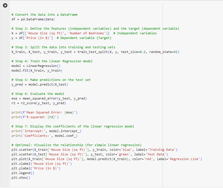
Explanation of Code:

1. Data Creation: We created a simple dataset of house sizes, the number of bedrooms, and house prices. The dataset is then converted into a Pandas DataFrame.
2. Feature Selection: We define X as the independent variables (house size and number of bedrooms) and y as the dependent variable (price).
3. Train-Test Split: The dataset is split into training and testing sets using the train_test_split function from scikit-learn. This ensures that we train the model on one part of the data and test it on unseen data to evaluate its performance.
4. Model Training: We use the LinearRegression model from scikit-learn to fit the training data. The model learns the relationship between the features and the target variable.
5. Prediction: The model is used to make predictions on the test set (X_test).
6. Model Evaluation: We evaluate the performance of the model using Mean Squared Error (MSE) and R-squared (R²). MSE tells us how far the predictions are from the actual values, and R² gives us a measure of how well the independent variables explain the variance in the dependent variable.
7. Coefficients and Intercept: The coefficients represent the weight of each feature, and the intercept represents the price when all features are zero.
8. Visualization (Optional): For simplicity, a scatter plot of house size and price is plotted, along with the regression line that fits the training data.

Interpreting the Results

• Coefficients: The coefficients tell us how much the house price changes for every unit increase in the features. For example, if the coefficient for house size is 200, it means that for every additional square foot, the price increases by $200.
• Mean Squared Error (MSE): The lower the MSE, the better the model is at predicting house prices. It tells us how close the predictions are to the actual prices.
• R-squared (R²): The R² score ranges from 0 to 1, where 1 indicates that the model explains 100% of the variance in the target variable. A score closer to 1 indicates a good fit.

Advantages of Linear Regression

1. Simplicity: Linear regression is easy to implement and interpret, making it a good starting point for regression tasks.
2. Efficiency: It works well with smaller datasets and less complex problems.
3. Interpretability: The relationship between the features and the target variable is easy to understand.

Limitations of Linear Regression

1. Assumes Linearity: Linear regression assumes that there is a linear relationship between the independent and dependent variables, which might not always be true.
2. Sensitive to Outliers: Outliers can significantly affect the performance of a linear regression model, leading to incorrect predictions.
3. Multicollinearity: If the independent variables are highly correlated with each other, the model’s coefficients can become unstable, making the results unreliable.

Conclusion

Linear regression is a powerful and easy-to-use algorithm that is widely applied in various fields, including finance, healthcare, and real estate. By understanding the relationship between the independent variables (features) and the dependent variable (target), linear regression can help us make informed predictions.